Features of Matrix eQTL

Matrix eQTL models

In addition to the standard additive linear model Matrix eQTL can search for eQTLs using two other models. The model is set by the useModel parameter of the main Matrix eQTL function Matrix_eQTL_main. All models are particular cases of linear regressions models. In the first, used in the sample code, the genotype is assumed to have only additive effect on expression:

Model: useModel = modelLINEAR
Equation: expression = α + ∑_k β_k⋅covariate_k + γ⋅genotype_additive
Testing for significance of: γ
Test statistic: t-statistic

Next model allows genotype to have both additive and dominant effects (ANOVA model). In this case genotype data set musts take at most 3 distinct values (i.e. 0/1/2/NA) unless specified otherwise. See modelANOVA page on how to change the number of ANOVA categories.

Model: useModel = modelANOVA
Equation: expression = α + ∑_k β_k⋅covariate_k + γ₁⋅genotype_additive + γ₂⋅genotype_dominant
Testing for significance of: (γ₁,γ₂) pair
Test statistic: F-statistic

Last but not least is the model testing for the significance of the interaction between the genotype and the last covariate. This model can be used to test for equality of effect sizes (as in the standard model) between two groups of samples (case vs. control). In this case the last covariate must be the dummy variable indicating the sample groups.

Model: useModel = modelLINEAR_CROSS
Equation:
expression = α + ∑_k β_k⋅covariate_k + γ⋅genotype_additive + δ⋅genotype_additive⋅covariate_K
Testing for significance of: δ
Test statistic: t-statistic

Correlated and heteroskedastic errors

Matrix eQTL supports linear models with correlated and/or heteroskedastic errors for all three types of linear models listed above. This feature may be useful when samples are known to have different quality or taken from related individuals.

To account for correlated or heteroskedastic errors set the parameter errorCovariance of the main function Matrix_eQTL_main to the error covariance matrix.

False discovery rate (FDR) estimation

Once Matrix eQTL discovers a set of significant gene-SNP pairs, it estimates a corresponding q-value (FDR) for each of them. The FDR is saved in the output files and in the object returned by Matrix_eQTL_main function. False discovery rate is estimated using Benjamini–Hochberg procedure under the assumption that the tests are 'independent or positively correlated', i.e. c(n) = 1.

It is the default behavior that Matrix_eQTL_main calculated FDR for the findings. However, to calculate FDR Matrix eQTL has to accumulate all significant results in computer memory. To turn off FDR calculation and reduce memory consumption one can set noFDRsaveMemory = TRUE in the call of the main function Matrix_eQTL_main.

Plotting p-value distribution

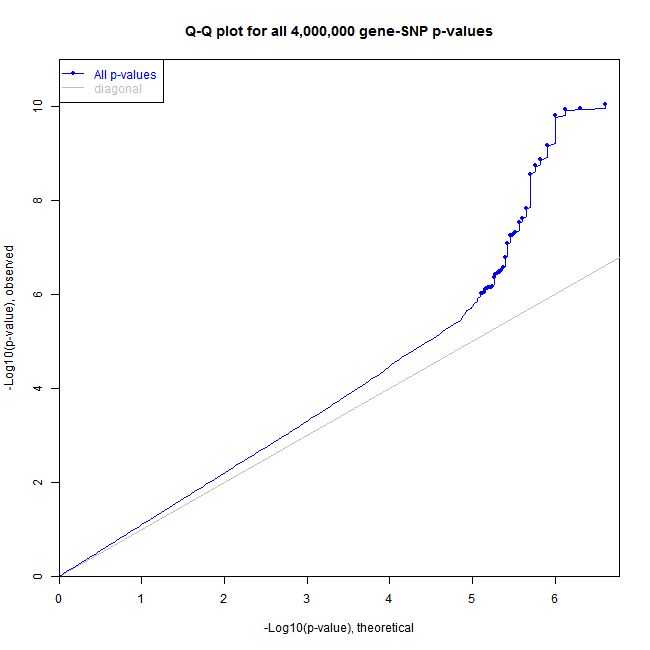
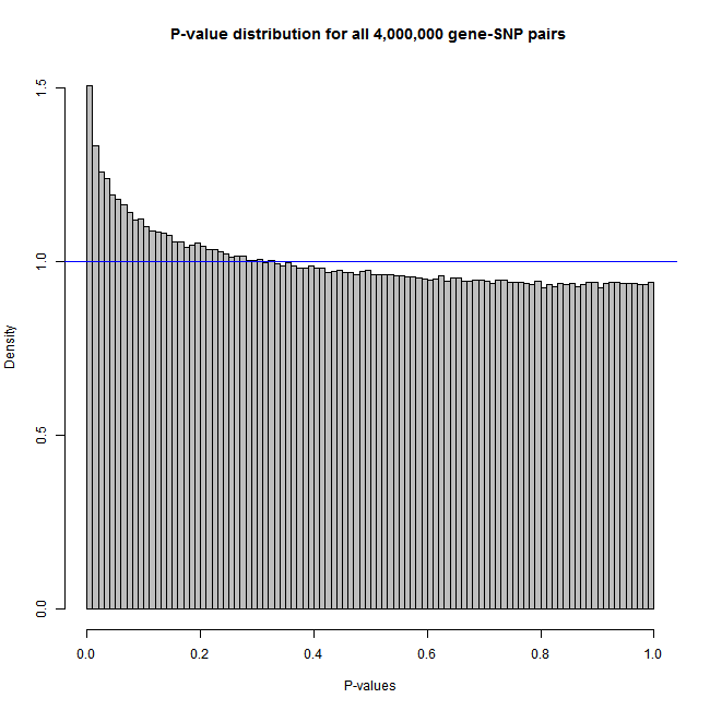
It is important to check eQTL results for inflation in the findings caused by unaccounted covariates, population stratification, plate effects, model misspecification, and other factors. A common approach for this check is to plot distribution of all recorded p-values on a QQ-plot or a histogram.

Matrix eQTL can record the distribution of p-values in all performed tests, even those that do not pass significance threshold and show it in a form of a QQ-plot or a histogram. To enable this feature change the parameter pvalue.hist of function Matrix_eQTL_main. The simple command plot applied to the output object of Matrix_eQTL_main function creates the requested plot. See the sample code for creating a histogram and a QQ-plot.

Here are the plots produced by the sample code:

• me = Matrix_eQTL_engine(..., pvalue.hist = "qqplot");
• plot(me, pch = 16, cex = 0.7);

QQ-plot for 4,000,000 p-values

• me = Matrix_eQTL_engine(..., pvalue.hist = 100);
• plot(me, col="grey");

Histogram of 4,000,000 p-values

Best p-value for each gene and each SNP (support for permutations)

Matrix eQTL can record the best p-value for each gene and each SNP even if these p-values do not beat the significance thresholds. This feature is useful for permutation analysis to assess significance of the best SNP for each gene or vice versa.

To turn on this feature set min.pv.by.genesnp = TRUE in the call of Matrix_eQTL_main.

The best p-values for each gene and each SNP are recorded in the output object of the main function Matrix_eQTL_main in some of the following elements: