Instruction for the use of Mixer: an improved method for ChIP-chip analysis by mixture model approach

Introduction

Mixer is a statistical framework for ChIP-chip or tiling array data analysis. It includes statistical methods for both data normalization and peak detection. The peak detection and quantification relies on a mixer model approach that dissects the distribution of background signals and the Immunoprecipitated signals. In contrast to many existing methods, mixer is more flexible by imposing less restrictive assumptions and allowing a relatively large proportion of peak regions. Robust performance on data sets predicted to contain numerous peaks is very important for the studies of the transcription factors with abundant binding sites, and common chromatin features or epigenetic marks.

Mixer is implemented as an R package. The source code includes both R and C codes. In this tutorial, we focus on using mixer for Nimblegen two-color array data. Similar methods can be applied to Affymetrix one-color array.

Download and Installation

The source code and binary versions for Windows/Mac can be downloaded here.

If the binary package cannot be installed (usually due to incompatible operation systems), install the source package. Since the R package contains C code, a C complier is required for installation.

Windows: Rtools need to be installed in order to Compile C codes in an R package. Please follow the Readme file in Rtools to set up the PATH variable. Most often R needs to be installed in c:/R.

Mac OSX: The C compiler can installed as part of the Xcode developer tool.

Linux: gcc compiler need to be installed

With both R and appropriate c complier installed, this R package can be installed as follows

(1) Open terminal in Mac or linux; Open a command prompt in Windows (Start menu -> run -> cmd, or Start menu -> cmd)

(2) Change to the directory where the source code is located. Untar the package using the command: tar –xzf mixer_version.tar.gz

(3) Install the package using the following command:

R CMD INSTALL mixer

Gather the Input Data

Mixer requires one information file and two data files. The following table describes these files. Data files have a “pair format”. The file with “_635” in its name corresponds to dye Cy5 and usually contains data from the IP sample. The file with “_532” in its name corresponds to dye Cy3 and usually contains data from the Control sample. For example, data listed in the following table can be downloaded from http://bioinformatics-renlab.ucsd.edu/rentrac/wiki/CTCF_Project

	Folder within Nimblegen CD	File type	Example
Information file	DesignFiles	.ndf	2005-05-10_HG17Tiling_Set25.ndf
Data file	PairData	.pair or .txt	41149_532_pair.txt, 41149_635_pair.txt

Using Mixer to Analyze Data

1. Read Data into R

R function read.table can be used to read in data. We suggest excluding the probes that are not from chromosome k, X or Y, where k is an integer. Mixer requires the probes to be sorted according to their chromosome and location.

library(mixer)

setwd("~/research/ChIP/demo")

info = read.table("DesignFiles/2005-05-10_HG17Tiling_Set25.ndf",

sep="\t", header=TRUE, as.is=TRUE)

info = info[grep("^(chr\\d+|chrX|chrY)$", info$SEQ_ID, perl=TRUE),]

info = info[order(info$SEQ_ID, info$POSITION),]

Cy3 = read.table("PairData/41149_532_pair.txt", sep="\t", header=TRUE)

Cy5 = read.table("PairData/41149_635_pair.txt", sep="\t", header=TRUE)

Note that usually the SEQ_ID column is chromosome. Occasionally, however, it may contain additional information. For example, in promoter arrays, it may resemble CHR10:100017497-100020197. In this case, extract the chromosome information from this column, for example, using “strplit” function as follows

seqSplit = strsplit(info$SEQ_ID, ":")

info$SEQ_ID = sapply(seqSplit, function(v){v[1]})

> info$SEQ_ID[1:2]

[1] "CHR10" "CHR10"

2. Align information and data

Since the information file and the data file may not have one-to-one correspondence, they may need to be aligned.

dataXY = paste(Cy5$X, Cy5$Y, sep="_")

infoXY = paste(info$X, info$Y, sep="_")

mat = match(infoXY, dataXY)

wNA = which(is.na(mat))

if(length(wNA) > 0){

info = info[-wNA,]

mat = mat[-wNA]

}

Cy5 = Cy5[mat,]

Cy3 = Cy3[mat,]

3. Normalize data

To normalize data, first calculate the GC content and then normalize the data based on the GC content. In the example code below, the parameter 50 in function code.AT.GC indicates that the probe sequences hvae length of 50 nt. See FAQ 1 in the event that probes have differing lengths.

seqGC = code.AT.GC(info$PROBE_SEQUENCE, 50)

nGC = apply(seqGC, 1, sum)

probeX = norm.GC(log2(Cy5$PM), log2(Cy3$PM), nGC, method="lowess")

4. Calculate probe-level and window-level local FDR

In the following R codes, pl and wl are probe-level and window-level local FDR, respectively. Two parameters must be specified for window level statistics calculation,s which are “radius” and “lambda”. The parameter lambda is set as 1 over the expected length of sonicated DNA fragments. In the example below, the expected fragment length is 1500bp (personal communication with Dr. Kim). Typically, the expected fragment length is from 500bp to1500bp. The parameter radius specifies the window size on each side of the probe for analysis. In this example, 500bp is used. Usually Radius can usually be chosen from the range of 300-500bp based on probe density and expected length of DNA fragments. For example, experiment with denser probes and shorter DNA fragments can have smaller radius, hence higher resolution.

pl = lfdr(probeX)

chr = info$SEQ_ID

probe.start = info$POSITION

probe.end = info$POSITION + 49

radius = 500

lambda = 1/1500

windowX = win(chr, probe.start, probe.end, probeX, pl,

lambda, radius)

wl = lfdr(windowX$x)

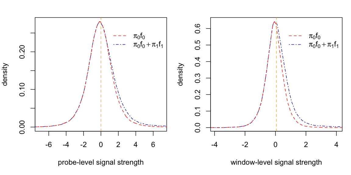
Function plot.lfdr plots the estimated density curves. The following figure depicts the density curves derived from the example data.

5. Merge peaks and output the results in gff format

Merge sliding windows around each of the probes into peak regions and output the results in gff formtat, wich can be visualized by Nimblegen SignalMap or the UCSC genome browser. Note that the “radius” and “lambda” parameters used for function mergeWindow should be the same as the ones used in function Win in step 5.

mpks = mergeWindow(windowX, wl, probeX, pl, radius, lambda,

window.cut=0.2, probe.cut.type="lfdr",probe.cut=1.0, n.probe=5)

gff(mpks, file="peaks.gff", source="Kim07", feature="41149_pks")

The following are examples of three peak regions in the output gff file. The columns are

chr11 Kim07 41149_pks 114700775 114701824 4.84 + . 11 0

chr11 Kim07 41149_pks 60361402 60362516 4.83 + . 5 0

chr11 Kim07 41149_pks 64906055 64907153 4.82 + . 7 6.4e-16

FAQ

1. How should data be normalized based on GC content if probes have different lengths?

One solution is to normalize by GC proportion. Transform GC proportions into integers over a range, for example 0 to 50.

seqLen = sapply(strsplit(info$PROBE_SEQUENCE, split=""), length)

seqGC = code.AT.GC(info$PROBE_SEQUENCE, seqLen)

nGC = round(50*apply(seqGC, 1, sum)/seqLen)

probeX = norm.GC(log2(Cy5$PM), log2(Cy3$PM), nGC, method="lowess")

2. How should replicates be handled?

Normalize the data for each array individually first. Then average the normalized intensity for each probe replicate. Finally, calculate probe-level/window-level lfdr using the average probe intensity.

Citation: Wei Sun, Michael J Buck, Mukund Patel and Ian J Davis (2009), Improved ChIP-chip analysis by mixture model approach.