Tutorial of genoCN [pdf]

A Brief Introduction

GenoCN is a software that simultaneously identify copy number states and genotype calls. Different strategies are implemented for the study of Copy Number Variations (CNVs) and Copy Number Aberrations (CNAs). While CNVs are naturally occurring and inheritable, CNAs are acquired somatic alterations most often observed in tumor tissues only. CNVs tend to be short and more sparsely located in the genome compared to CNAs. GenoCN consists of two components, genoCNV and genoCNA, designed for CNV and CNA studies, respectively. In contrast to most existing methods, genoCN is more flexible in that the model parameters are estimated from the data instead of being decided a priori. genoCNA also incorporates two important strategies for CNA studies. First, the effects of tissue contamination are explicitly modeled. Second, if SNP arrays are performed for both tumor and normal tissues of one individual, the genotype calls from normal tissue are used to study CNAs in tumor tissue.

Download and Installation

The source code and binary versions for Windows/Mac can be downloaded here.

If the binary package cannot be installed (usually due to incompatible operation systems), install the source package. Since the R package contains C code, a C complier is required for installation.

Windows: Rtools need to be installed in order to Compile C codes in an R package. Please follow the Readme file in Rtools to set up the PATH variable. Most often R needs to be installed in c:/R.

Mac OSX: The C compiler can installed as part of the Xcode developer tool.

Linux: gcc compiler need to be installed

With both R and appropriate c complier installed, this R package can be installed as follows

(1) Open terminal in Mac or Linux; Open a command prompt in Windows (Start menu -> run -> cmd, or Start menu -> cmd)

(2) Change to the directory where the source code is located. Untar the package using the command: tar –xzf genoCN_version.tar.gz

(3) Install the package using the following command:

R CMD INSTALL genoCN

1. genoCNV: an Example Using Simulated Data

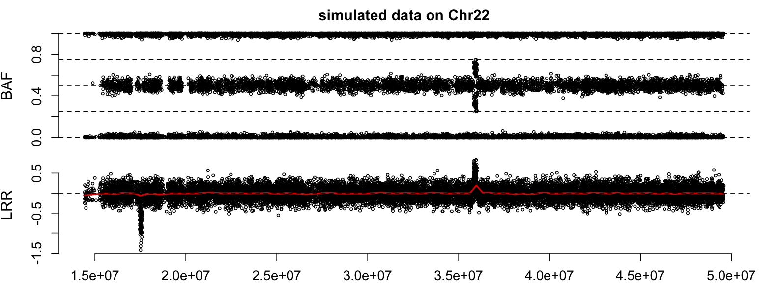
We first illustrate the usage of genoCNV by a simulated data. Specifically, we simulated LRR and BAF data for 17,348 SNPs on chromosome 22. Two CNVs are simulated. One is from the 1001-th probe to the 1100-th probe, with copy number 1. The other one is from the 10,001-th probe to the 10,200-th probe, with copy number 3.

First, load the SNP data and SNP information into R workspace, and check the dimensions and a few rows of the data.

data(snpData)

data(snpInfo)

dim(snpData)

dim(snpInfo)

snpData[1:2,]

snpInfo[1:2,]

For each SNP, the information we need includes its name, chromosome, position and population frequency of B allele (PFB). Some processed SNP information files can be found in PennCNV package: http://www.openbioinformatics.org/ penncnv/penncnv_download.html. The data of each SNP includes LRR and BAF. Next, we suggest plot the LRR and BAF values for at least a few samples on a few chromosome to double check the data.

plotCN(pos=snpInfo$Position, LRR=snpData$LRR, BAF=snpData$BAF,

main = "simulated data on Chr22")

Next, run genoCNV to identify CNV regions.

Theta = genoCNV(snpInfo$Name, snpInfo$Chr, snpInfo$Position, snpData$LRR, snpData$BAF,

snpInfo$PFB, sampleID="simu1", cnv.only=(snpInfo$PFB>1), outputSeg = TRUE,

outputSNP = 1, outputTag = "simu1")

where the first three parameters provide the SNP information and the next three parameters provide SNP data. The parameter "cnv.only" is an indicator variable for the “copy-number-only probes”. Those probes do not overlap with any SNPs, so there is only one allele, and the measurement of BAF is not informative. We only use the LRR information for those “copy-number-only probe”. In practice, we decide whether a probe is copy-number-only by checking whether its population frequency of B allele (PFB) is larger than 1.

The function genoCNV returns a list (e.g., "Theta" in the above example), which includes the estimates of all the parameters. By specifying "outputSeg=TRUE", the information of the copy number altered regions are written into a text file named "TAG_segment.txt", where "TAG" is specified by the parameter "outputTag". The parameter "outputSNP" specifies the the output of SNP-specific information.

· If "outputSNP"=0, do not output SNP-specific information.

· If "outputSNP" is 1, output the most likely copy number and genotype state of the SNPs that are within copy number altered regions.

· If "outputSNP" is 2, output the most likely copy number and genotype state of all the SNPs (whether it is within CNV regions or not).

· If "outputSNP" is 3, output the posterior probability for all the copy number and genotype states for the SNPs.

In the output file “simu1_segment.txt”, "chr", "start", and "end" specify the chromosome location of copy number altered region. "state" is the state in the HMM. "sample" is the sample ID. "snp1" and "snp2" are the two flanking SNPs of the copy number altered region. "score" is the summation of posterior probability of the SNPs within the region, and "n" is the number of SNPs within the region. Note: by default, only the segments with at least 3 SNPs are output to segment file. This cutoff can be controlled by the parameter "seg.nSNP". The following codes show part of the snp file:

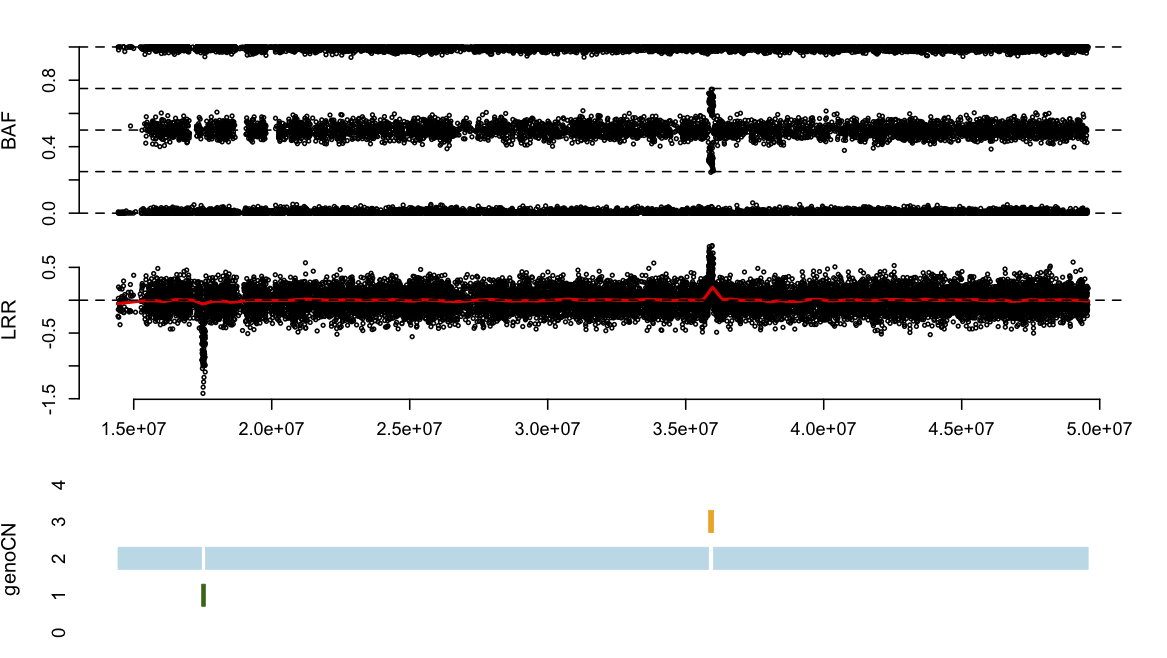
Finally, plot the copy number call results by genoCN, as is shown in Figure 2. It is very important to examine the copy number calls by this type of figures to validate the results. Note, the file name provided to function plot CN is the name of segment output file, instead of snp output file.

plotCN(pos=snpInfo$Position, LRR=snpData$LRR, BAF=snpData$BAF,

main = "simulated data on Chr22", fileNames="simu1_segment.txt")

2. genoCNV: a typical case of real data study

In a real data study, some preliminary data processing is necessary. We will illustrate an typical case of real data study in this section.

2.1 Read Data into R

First, read the information of all the SNPs into R, for example:

info = read.table("snp_info_hg18.txt", header=TRUE, sep="\t", as.is=TRUE)

The first a few lines of this information file is as following:

Name Chr Position PFB

1 rs12354060 1 10004 1

2 rs2691310 1 46844 0

Next, read the data of one sample into R. For example,

dat = read.table("NA06993.txt", sep=",", header=TRUE, as.is=TRUE)

Here we use the data file NA06993.txt that includes the data for a Hapmap individual. This data is available to direct customers of Illumina through their iCom account. The first a few rows of this file is shown below:

Name Sample Allele1 Allele2 GCScore X Y XRaw YRaw LRR BAF

1 200003 NA06993 G G 0.9299 0.072 0.902 1113 11326 0.0180 0.9821

2 200006 NA06993 T T 0.7877 1.669 0.152 13324 2429 -0.0154 0.0099

Note that we just need three columns in this data file: "Name", "LRR", and "BAF".

2.2 Align Information and Data

The rows of information and the data may not be one-to-one correspondence. We need to align them. Here we just look at chromosome 1 to 22. \textbf{Note:} the input data for genoCNV or genoCNA must be sorted by their chromosomal locations. In this example, the probes are already sorted by their chromosomal locations in the information file and we simply re-order the rows in the data according to their order in information file.

if(any(! dat$Name %in% info$Name)){

stop("missing SNP information \n")

}

mt = match(info$Name, dat$Name)

wNA = which(is.na(mt))

if(length(wNA)>0){

info = info[-wNA,]

mt = mt[-wNA]

}

dat = dat[mt,]

wkp = which(info$Chr %in% as.character(1:22))

dat = dat[wkp,]

info = info[wkp,]

2.3 Run genoCNV

We can run genoCNV using a sample code like the following:

Theta = genoCNV(info$Name, info$Chr, info$Position, dat$LRR, dat$BAF,

info$PFB, sampleID="NA06993", cnv.only=(info$PFB>1), outputSeg = TRUE,

outputSNP = 1, outputTag = "NA06993")

3. genoCNA

Usage of function “genoCNA” is similar to “genoCNV”. There are three extra parameters for genoCNA:

1. Contamination: whether we model tissue contamination, the default value is TRUE.

2. NormalGtp: normalGtp is specified only if paired tumor-normal SNP array is available. It is the normal tissue genotype for all the SNPs specified in snpNames, which can only take four different values: -1, 0, 1, and 2. Values 0, 1, 2 correspond to the number of B alleles, and value -1 indicates the normal genotype is missing. By default, it is NULL, means no genotype from normal tissue.

3. Geno.error: probability of genotyping error in normal tissue genotypes. The default value is 0.01.

3.1 Estimate tumor purity from the output genoCNA

Suppose the finial parameter estimates are Theta1. We need to use the mu.b component of Theta1, which are estimates of the mean values of the BAF distributions. mu.b is a matrix of nine rows and four columns. For example:

$mu.b

[,1] [,2] [,3] [,4]

[1,] 0.0 0.500 1.000 NA

[2,] 0.0 0.100 0.900 1

[3,] 0.5 NA NA NA

[4,] 0.0 0.170 0.830 1

[5,] 0.0 0.340 0.660 1

[6,] 0.0 0.070 0.930 1

[7,] 0.0 0.500 1.000 NA

[8,] 0.0 0.055 0.945 1

[9,] 0.0 0.250 0.750 1

Each row of mu.b corresponds to one state of the HMM, and the states are ordered as in Table 2 of Sun et al. (2009). Within each row, genotype classes are also ordered as in Table 2 of Sun et al. (2009). An NA in the above matrix indicates an unused table cell. The following code is an example to estimate tumor purity using the BAF of the homozygous deletion state.

# the BAF for the genotype mixture of (A, AB) and (B, AB), where AB is from normal tissue.

Beta.A.AB = Theta1$mu.b[4,2]

Beta.B.AB = Theta1$mu.b[4,3]

# the BAF for genotype AB

Beta.AB = Theta$mu.b[1,2]

# Update BAF estimates to take into account of systematic dye bias

# this step is not necessary if there is no systematic bias

Beta.A.AB = 0.5*Beta.A.AB/Beta.AB

Beta.B.AB = 0.5 + 0.5*(Beta.B.AB - Beta.AB)/(1 - Beta.AB)

# Re-estimate Beta.A.AB by averaging Beta.A.AB and 1 - Beta.B.AB

Beta1 = 0.5*(Beta.A.AB + 1 - Beta.B.AB)

# estimate tumor purity, since we examine the genotype A, nA = 1 and nB = 0

nA = 1

nB = 0

pT = (1 - 2*Beta1)/(Beta1*(nA + nB - 2) + 1 - nB)

# Note, in the earlier version of this help page, we have a typo,

# we mistakenly wrote the denominator as Beta1*(nA + nB - 2) + 1 – nB.

# We apologize for that. All the results in our paper are based on the correct formula.

4. FAQ

4.1. How long does it take for genoCN to run one sample?

Typically, for an array with 1 million probes, it takes 2 to 5 minutes.

4.2. How much memory does genoCN need?

To run an array with 1 million probes, genoCN typically takes less than 2G memories, which is affordable for most 32-bit machines.

4.3. Can I run genoCN on Affymetrix Array?

Yes. However, you need to generate LRR/BAF from Affymetrix SNP array data. PennCNV-Affy is one available tool to do so (http://www.openbioinformatics.org/penncnv/penncnv_tutorial_affy_gw6.html). We are working on a more advanced method to normalize the output of Affymetrix array to obtain LRR and BAF.

4.4. Can I reduce the computational burden by avoiding the parameter estimation?

Yes, you can. First, it is strongly not recommended to use fixed parameter for CNA analysis. Secondly, for CNV analysis, “fixed parameter” option usually leads to less CNV regions, but slightly higher specificity.

There are two relevant parameters in genoCNV/genoCNA for this purpose: ‘Para’ and ‘fixPara’.

The parameter ‘Para’ specifies a list of initial parameters for the HMM. If Para is NULL, the default initial parameters: init.Para.CNV/init.Para.CNA is used. init.Para.CNV and init.Para.CNA are data stored in the R package. In the subfolder named 'test' of the R package, there is R code to generate the initial parameter estimates.

If fixPara=TRUE, genoCN will use the initial parameters for the computation without estimating it.

There is certainly an option to use a subset of samples in your study to estimate the parameters. If the resulting parameters are similar across the subset of samples, you can take mean or median of the parameter estimates and use them as fixed parameters to run all the other samples.

4.5. I got the output of of SNP-wise information from my output file ‘sample1_SNP.txt’, as is shown below.

name state stateP CN CNP genotype genoP

rs8179466 3 0.9993816 0 0.9993816 Null 0.9993816

....

cnvi0007379 5 0.6929201 3 0.6929201 NA NA

....

rs13303118 2 0.9893327 2 0.9893327 AABB 0.0105861

I had three questions. First, what does genotype ‘Null’ means? Secondly, why the genotype of cnvi0007379 is ‘NA’? Thirdly, for SNP rs13303118, why the most likely copy number is 2, but the most likely genotype is AABB?

First, the genotype Null means there is complete deletion so this part of DNA sequence does not exist in this specific individual (or, you can say this is an amplification in the reference genome).

Secondly, cnvi0007379 is a copy number probe, so we only use its LRR, but not BAF in the genoCN, so there is no genotype output. In fact, there is no need to have genotype output since the genotype from all the individuals will be the same.

Thirdly, it is possible that the copy number of the most likely genotype is different from the most likely copy number. I will try to explain it two examples.

(1) The most likely state is state 1 (AA, AB, BB) which has posterior probability 0.6. This probability can be decomposed to four parts (not three parts): the probability for AA, AB, BB, and the background component. It is possible that each of them has a relatively small probability, say smaller than 0.2. While the probability for genotype AAB is 0.39. Then the most likely genotype is AAB.

(2) The most likely copy number is 2, but the most likely state is state 2 (LOH with only possible genotypes as AA and BB). Now the probability of genotype AB is small since the probability of state 1 (AA, AB, BB) is small. It is possible that other genotype, say AABB, has highest probability. This is the situation for rs13303118 in the above output.

Well, we have explanations, but we still do not like this inconsistency. This inconsistency can be avoided by simply requiring the posterior probability larger than 0.5 for either copy number or genotype, otherwise set the copy number or genotype as missing.

Citation: Sun, W., Wright , F., Tang, Z.Z., Nordgard , S.H., Van Loo, P., Yu, T., Kristensen, V., Perou, C., Integrated study of copy number states and genotype calls using high density SNP arrays.Nucleic Acids Res. 2009, 37(16), 5365-77